Principio di indeterminazione …

Principio di indeterminazione di Heisenberg
Werner Karl Heisenberg è stato un fisico tedesco nato a Würzburg il 5 dicembre 1901 e morì il 1° febbraio 1976. Fu tra gli scienziati protagonisti nello studio e approfondimento della Meccanica Quantistica e nel 1925 pubblicò articoli sulla “Meccanica delle Matrici” e nel 1927 il “principio di indeterminazione” per il quale ottenne il premio Nobel nel 1932 [1]. Il principio di indeterminazione di Hisemberg stabilisce il limite della precisione nella misurazione in un sistema fisico [2]. Tale principio si colloca nella determinazione di valori a grandezze fisiche simultaneamente per comprenderne l’attendibilità e la precisione [3].
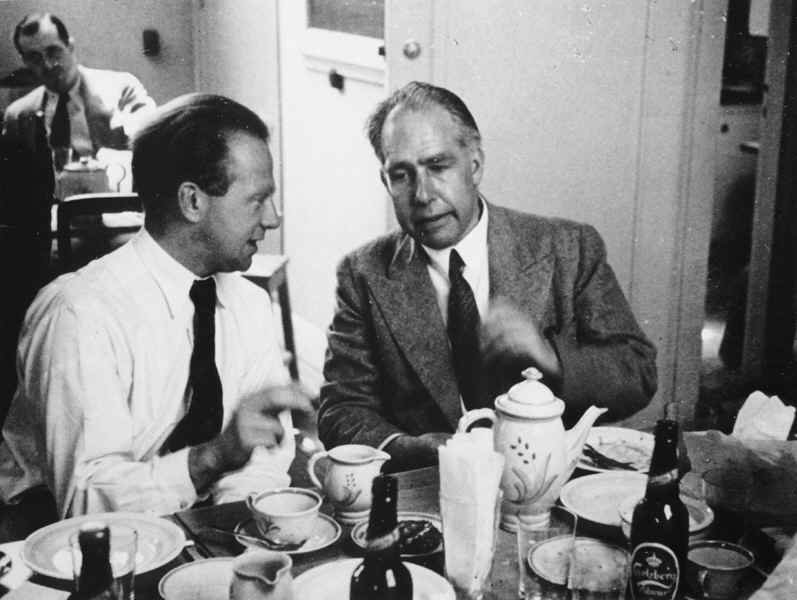
Figura 1 – Heisenberg e Bohr – Di Fermilab, U.S. Department of Energy – http://www.fnal.gov/pub/inquiring/timeline/images/heisenbergbohr.jpg shown on http://www.fnal.gov/pub/inquiring/timeline/05.html, Pubblico dominio, https://commons.wikimedia.org/w/index.php?curid=6877522
Le incertezze vengono poste come limite fisico dei sistemi e il dualismo onda-particella spiega in modo esemplare le caratteristiche del principio di indeterminazione [4], infatti la validità è molto più evidente nei corpi microscopici ovvero compatibili con la lunghezza d’onda della radiazione elettromagnetica incidente sul corpo stesso. Il metodo molto spesso utilizzato per determinare la posizione utilizza una radiazione elettromagnetica monocromatica incidente sul corpo e la relativa radiazione diffusa per misurare la posizione. Supponiamo di irradiare un microscopico corpo con radiazione di 500 nm e la denominiamo λ1 con risultante incertezza Δx1; successivamente lo stesso corpo lo investiamo con radiazione elettromagnetica di 100 nm (λ2) e misurazione Δx2. Pertanto: Δx1∼ λ1 e Δx2 ∼ λ2 e facendo rapporto tra (Δx1/ Δx2) = (λ1/ λ2) = 5 – ovvero utilizzando prima la radiazione di 500 nm e dopo da 100 nm otteniamo una diminuzione dell’incertezza iniziale di 5 volte.
Probability densities corresponding to the wave functions of an electron in a hydrogen atom possessing definite energy levels….
La misura dei momenti lineari Pxn si possono effettuare se noti massa e velocità. Per misurare la velocità possiamo determinare la posizione in due tempi successivi (X1(t1)) e (X2(t2)) e se utilizzo fotoni avremo momento h/ λ – la diffusione creata dall’impatto dei fotoni con l’oggetto cambierà il momento lineare in modo indeterminato. Utilizzando prima λ1=500nm e successivamente λ2=100 possiamo verificare rapporti (Δp1/ Δp2) = ((h/ λ1)/(h/ λ2)) = λ2/ λ1 = 1/5. Questo risultato porta a conclusioni opposte rispetto alla posizione, ovvero che la diminuzione della lunghezza d’onda della radiazione elettromagnetica incidente conduce a aumento errore nel momento lineare di 5 volte e errore nella posizione a 1/5. In formula possiamo rappresentarlo con Δx Δpx≥ (1/2) ℏ [5]. Questo è un approccio semiquantistico e per completezza è opportuno arrivare alle stesse conclusioni con punto di vista quantistico. Il primo postulato della meccanica quantistica riportato da Melvin W Hanna [6] recita quanto segue: “Ogni stato di un sistema dinamico costituito da N particelle è descritto dal modo più completo possibile da una funzione Ѱ (q1,q2,……,qn,t) tale che Ѱ*Ѱ dτ è proporzionale alla probabilità di trovare q1 nell’intervallo compreso tra q1 e q1+ dq1; q2 nell’intervallo q2 e q2+dq2 …… al tempo dato t”. Questo postulato propone di calcolare la probabilità di determinare la particella in esame utilizzando la soluzione dell’equazione di Schrödinger della particella Ѱ=(Ae^ikx) e quindi Ѱ*Ѱ=(Ae^ikx) (Ae^-ikx) = A^2 . Questo risultato dice che esiste una equiprobabilità di trovare la particella quindi se è determinato il momento lineare in x è impossibile determinare la posizione della particella sull’asse x. [7]
————————————-
Heisenberg’s uncertainty principle
Werner Karl Heisenberg [figure 1] was a German physicist born in Würzburg on December 5, 1901 and died on February 1, 1976. He was one of the leading scientists in the study and in-depth study of Quantum Mechanics and in 1925 he published articles on “Matrix Mechanics” and in 1927 the “Uncertainty principle” for which he received the Nobel Prize in 1932 [1]. Hisemberg’s uncertainty principle establishes the limit of measurement accuracy in a physical system [2]. This principle is placed in the determination of values of physical quantities simultaneously to understand their reliability and precision [3]. Uncertainties are placed as the physical limit of the systems and the wave-particle dualism explains in an exemplary way the characteristics of the uncertainty principle [4], in fact the validity is much more evident in microscopic bodies, i.e. compatible with the wavelength of electromagnetic radiation accident on the body itself. The method very often used to determine the position uses monochromatic electromagnetic radiation incident on the body and the related scattered radiation to measure the position. Suppose we irradiate a microscopic body with 500 nm radiation and we name it λ1 with resulting uncertainty Δx1; subsequently we hit the same body with electromagnetic radiation of 100 nm (λ2) and measurement Δx2. Therefore: Δx1∼ λ1 and Δx2 ∼ λ2 and making the ratio between (Δx1 / Δx2) = (λ1 / λ2) = 5 – or using first the radiation of 500 nm and then from 100 nm we obtain a decrease of the initial uncertainty of 5 times .The measurement of linear moments Pxn can be performed if mass and velocity are known. To measure the speed we can determine the position in two successive times (X1 (t1)) and (X2 (t2)) and if I use photons we will have moment h / λ – the diffusion created by the impact of the photons with the object will change the moment linear indefinitely. Using first λ1 = 500nm and then λ2 = 100 we can verify ratios (Δp1 / Δp2) = ((h / λ1) / (h / λ2)) = λ2 / λ1 = 1/5. This result leads to opposite conclusions with respect to the position, namely that the decrease in the wavelength of the incident electromagnetic radiation leads to an increase in the linear momentum error of 5 times and an error in the position at 1/5. In formula we can represent it with Δx Δpx≥ (1/2) ℏ [5]. This is a semiquantistic approach and for completeness it is appropriate to arrive at the same conclusions from a quantum point of view. The first postulate of quantum mechanics reported by Melvin W Hanna [6] reads as follows: “Each state of a dynamic system consisting of N particles is described as completely as possible by a function Ѱ (q1, q2, ……, qn, t) such that Ѱ * Ѱ dτ is proportional to the probability of finding q1 in the interval between q1 and q1 + dq1; q2 in the interval q2 and q2 + dq2 ……. at the given time t “. This postulate proposes to calculate the probability of determining the particle under consideration using the solution of the Schrödinger equation of the particle Ѱ = (Ae ^ ikx) and therefore Ѱ * Ѱ = (Ae ^ ikx) (Ae ^ -ikx) = A ^ 2 . This result says that there is an equiprobability of finding the particle so if the linear moment in x is determined it is impossible to determine the position of the particle on the x axis [7].
Figura 1 – Heisenberg e Bohr – Di Fermilab, U.S. Department of Energy – http://www.fnal.gov/pub/inquiring/timeline/images/heisenbergbohr.jpg shown on http://www.fnal.gov/pub/inquiring/timeline/05.html, Pubblico dominio, https://commons.wikimedia.org/w/index.php?curid=6877522
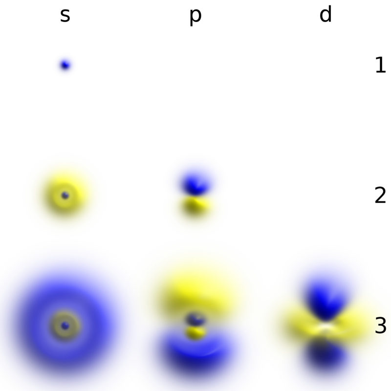
Figura 2: Probability densities corresponding to the wave functions of an electron in a hydrogen atom possessing definite energy levels (increasing from the top of the image to the bottom: n = 1, 2, 3, …) and angular momenta (increasing across from left to right: s, p, d, …). Denser areas correspond to higher probability density in a position measurement. Such wave functions are directly comparable to Chladni’s figures of acoustic modes of vibration in classical physics and are modes of oscillation as well, possessing a sharp energy and thus, a definite frequency. The angular momentum and energy are quantized and take only discrete values like those shown (as is the case for resonant frequencies in acoustics) – By Geek3 – Own work; created with hydrogen-cloud in Python This PNG graphic was created with Python., CC BY-SA 4.0, https://commons.wikimedia.org/w/index.php?curid=69032672;
Bibliografia
[1] https://it.wikipedia.org/wiki/Werner_Karl_Heisenberg;
[2] https://it.wikipedia.org/wiki/Principio_di_indeterminazione_di_Heisenberg;
[3] https://en.wikipedia.org/wiki/Uncertainty_principle;
[4] https://de.wikipedia.org/wiki/Heisenbergsche_Unsch%C3%A4rferelation;
[5] Corso di Fisica – Paul A. Tipler – Gene Mosca – 2010 – Quarta edizione italiana condotta sulla sesta edizione americana – ZANICHELLI;
[6] Chimica e Meccanica Quantistica – Melvin W. Hanna – 1974 – edizione italiana a cura di Aldo Gamba – casa editrice Ambrosiana;
[7] Chimica Fisica – Peter W. Atkins – 1993 – seconda edizione italiana condotta sulla terza edizione originale.
Dedicato a una persona a me molto cara di nome Pierrenata,
Lo dedico inoltre al prof Basosi Riccardo, una roccaforte internazionale della chimica fisica
Dr. Riccardo Zanaboni (Esponente del Comitato Scientifico del Centro Italiano Ricerche)
By: C.I.R. Centro Italiano Ricerche